Quickstart
Here’s how to get up and running with specmatch-emp
Library
specmatch-emp comes with a large library high-resolution optical
spectra shifted onto the rest wavelength scale. We’ll import the
library, along with some other useful modules.
import pandas as pd
from pylab import *
import specmatchemp.library
import specmatchemp.plots as smplot
Now we’ll load in the library around the Mgb triplet. By default,
SpecMatch create the following directory ${HOME}/.specmatchemp/ and
download the library into it.
lib = specmatchemp.library.read_hdf(wavlim=[5140,5200])
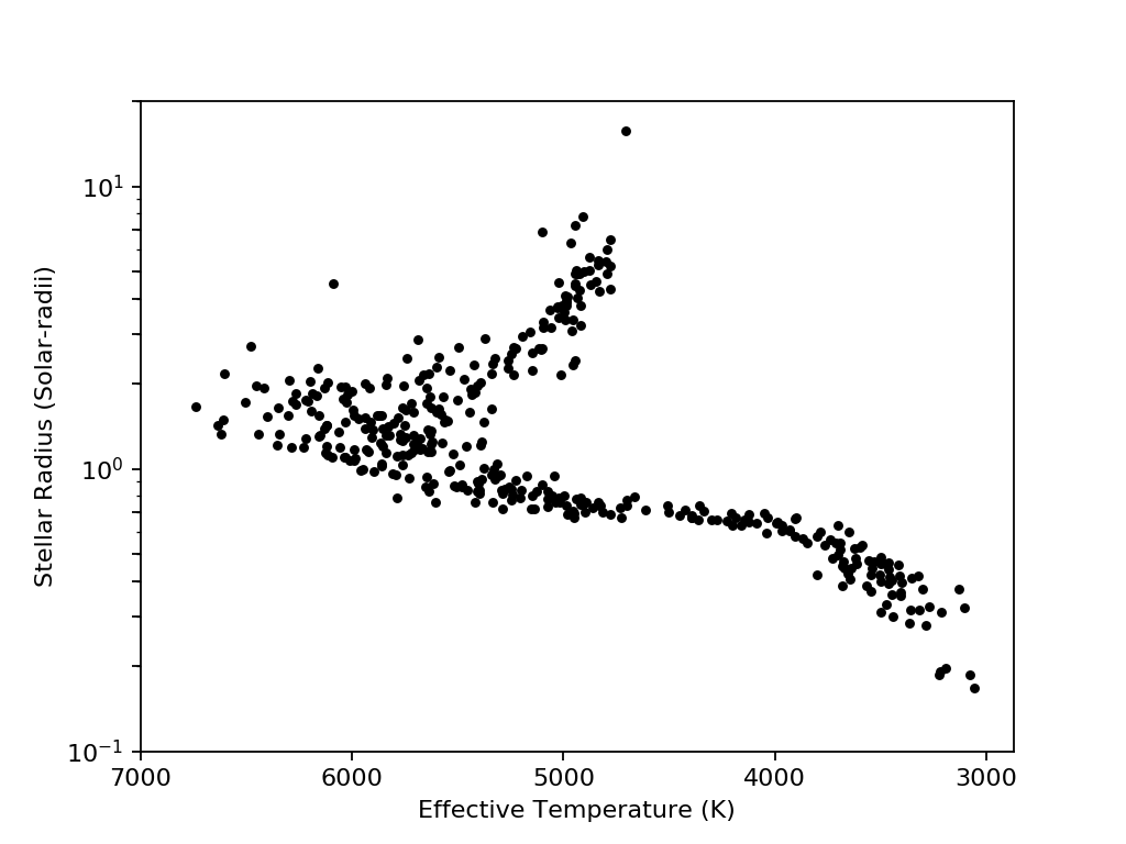
Here’s how the library spans the HR diagram.
fig = figure()
plot(lib.library_params.Teff, lib.library_params.radius,'k.',)
smplot.label_axes('Teff','radius')
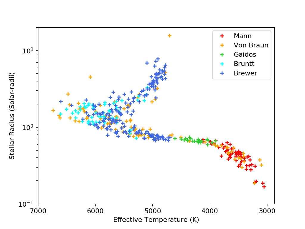
And here’s the library with the sources labeled.
fig = figure()
g = lib.library_params.groupby('source')
colors = ['Red','Orange','LimeGreen','Cyan','RoyalBlue','Magenta','ForestGreen']
i = 0
for source, idx in g.groups.items():
    cut = lib.library_params.ix[idx]
    color = colors[i]
    plot(
        cut.Teff, cut.radius,'+', label=source, color=color, alpha=1, ms=5,
        mew=1.5
    )
    i+=1
legend()
smplot.label_axes('Teff','radius')
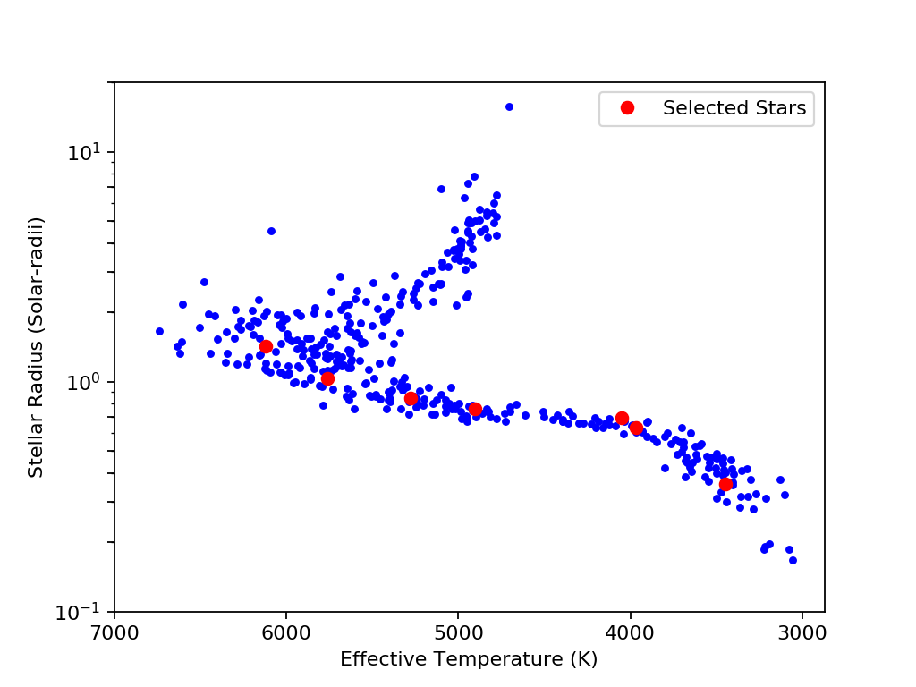
The parameters are stored in a pandas DataFrame which makes querying easy. Let’s grab some representative dwarf star spectra.
cut = lib.library_params.query('radius < 1.5 and -0.25 < feh < 0.25')
g = cut.groupby(pd.cut(cut.Teff,bins=arange(3000,7000,500)))
cut = g.first()

fig = figure()
plot(lib.library_params.Teff, lib.library_params.radius,'b.', label='_nolegend_')
plot(cut.Teff, cut.radius,'ro', label='Selected Stars')
legend()
smplot.label_axes('Teff','radius')
fig.savefig('quickstart-library-selected-stars.png')
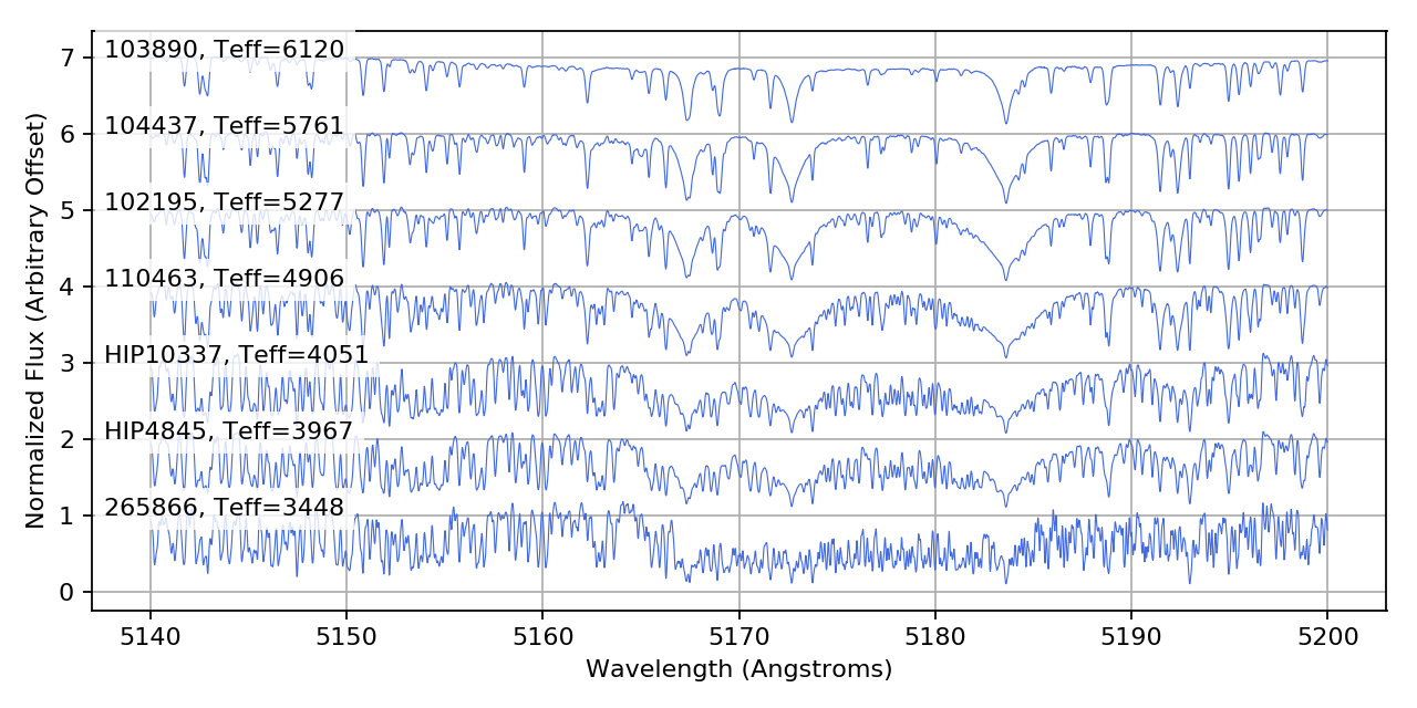
Plot the Mgb region for the spectra sorted by effective temperature
from matplotlib.transforms import blended_transform_factory
fig,ax = subplots(figsize=(8,4))
trans = blended_transform_factory(ax.transAxes,ax.transData)
bbox = dict(facecolor='white', edgecolor='none',alpha=0.8)
step = 1
shift = 0
for _,row in cut.iterrows():
    spec = lib.library_spectra[row.lib_index,0,:]
    plot(lib.wav,spec.T + shift,color='RoyalBlue',lw=0.5)
    s = "{cps_name:s}, Teff={Teff:.0f}".format(**row)
    text(0.01, 1+shift, s, bbox=bbox, transform=trans)
    shift+=step

grid()
xlabel('Wavelength (Angstroms)')
ylabel('Normalized Flux (Arbitrary Offset)')
Shifting
In the rest of this document, we will look at two example stars: HD 190406 (spectral class G0V), and Barnard’s star (GL 699), an M dwarf. Both of these stars are already in our library, so we will remove them from the library.
idx1 = lib.get_index('190406')
G_star = lib.pop(idx1)
idx2 = lib.get_index('GL699')
M_star = lib.pop(idx2)
To begin using SpecMatch, we first load in a spectrum and shift it onto the library wavelength scale. The raw HIRES spectra have been provided in the samples folder.
We read in the spectrum of HD 190406, in the same wavelength region as the library.
from specmatchemp import spectrum
G_spectrum = spectrum.read_hires_fits('../samples/rj59.1923.fits').cut(5130,5210)
G_spectrum.name = 'HD190406'
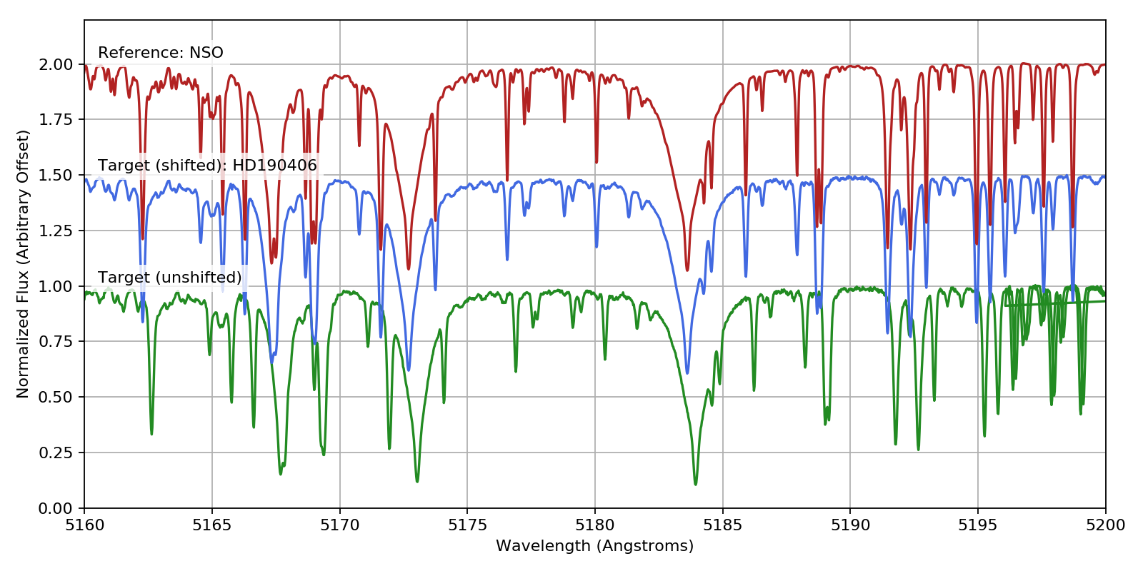
To shift the spectrum, we create the SpecMatch object and run shift().
This method runs a cross-correlation between the target spectrum and several reference spectra in the library for a select region of the spectrum. The reference spectrum which gives the largest cross-correlation peak is then used to shift the entire spectrum.
from specmatchemp.specmatch import SpecMatch
sm_G = SpecMatch(G_spectrum, lib)
sm_G.shift()
We can see the results of the shifting process. In this case, the code chose to use the NSO spectrum as the reference. We make use of the spectrum.Spectrum.plot() method to quickly plot each of the unshifted, shifted and reference spectra. Note that HIRES has overlapping orders so some spectral lines appear twice. In the final resampled spectrum, the small segments of overlapping orders are averaged.
fig = plt.figure(figsize=(10,5))
sm_G.target_unshifted.plot(normalize=True, plt_kw={'color':'forestgreen'}, text='Target (unshifted)')
sm_G.target.plot(offset=0.5, plt_kw={'color':'royalblue'}, text='Target (shifted): HD190406')
sm_G.shift_ref.plot(offset=1, plt_kw={'color':'firebrick'}, text='Reference: '+sm_G.shift_ref.name)
plt.xlim(5160,5200)
plt.ylim(0,2.2)
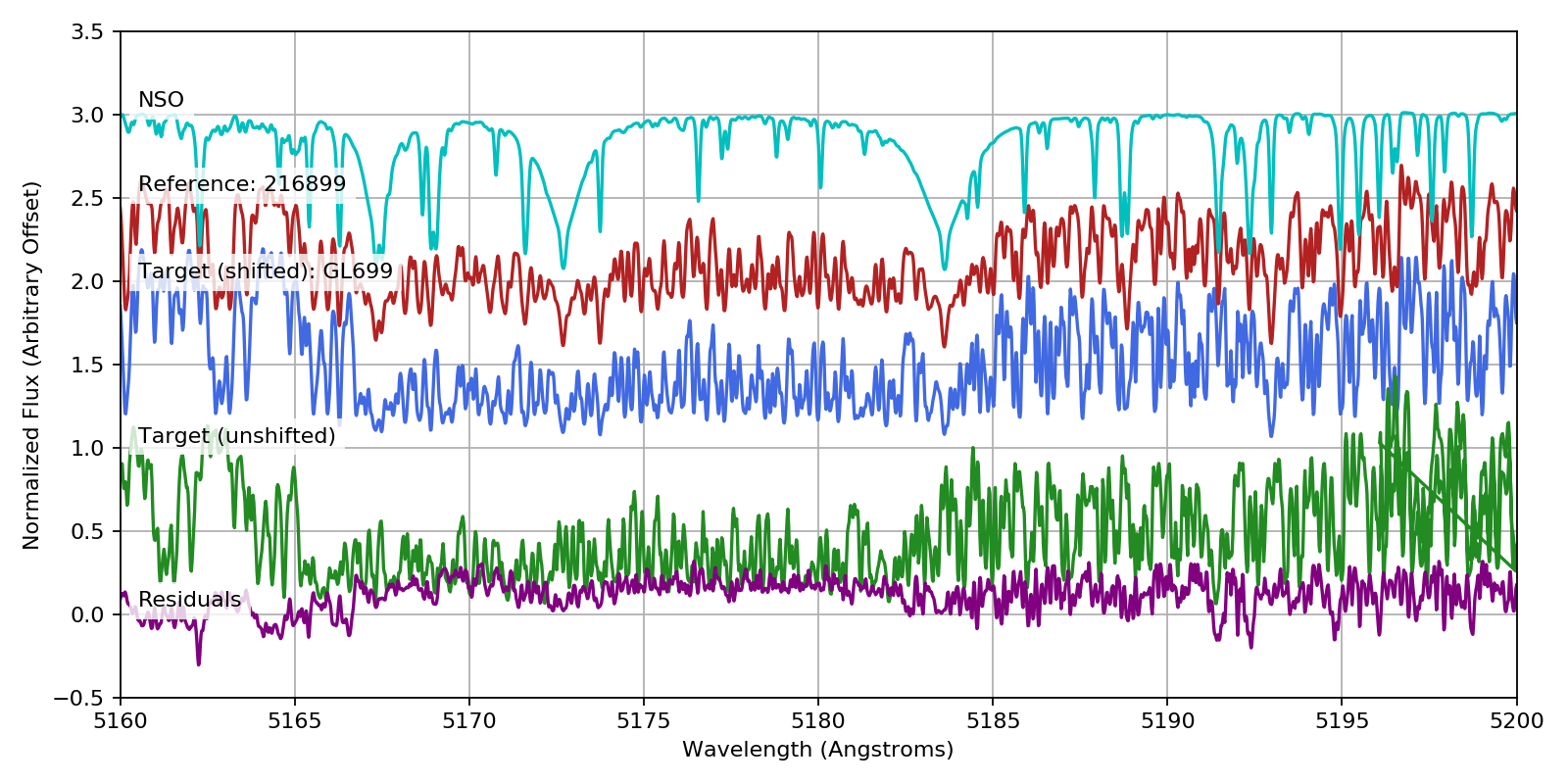
We repeat the same process for the M star spectrum. In this case, we see
that the code chose to shift the spectrum to a different reference: HD216899,
which is another M dwarf in our library. We have used the convenience
function SpecMatch.plot_shifted_spectrum() to easily plot
the shift results.
# Load spectrum
M_spectrum = spectrum.read_hires_fits('../samples/rj130.2075.fits').cut(5130,5210)
M_spectrum.name = 'GL699'

# Shift spectrum
sm_M = SpecMatch(M_spectrum, lib)
sm_M.shift()

# Plot shifts
fig = plt.figure(figsize=(10, 5))
sm_M.plot_shifted_spectrum(wavlim=(5160, 5200))
Matching
Now, we can perform the match. We first run SpecMatch.match(), which
performs a match between the target and every other star in the library,
allowing v sin i to float and fitting a spline to the continuum.
We can then plot the chi-squared surfaces to see where the best matches lie in parameter space.
sm_G.match(wavlim=(5140,5200))

# Plot chi-squared surfaces
fig = figure(figsize=(12, 8))
sm_G.plot_chi_squared_surface()
# Indicate library parameters for target star.
axes = fig.axes
axes[0].axvline(G_star[0]['Teff'], color='k')
axes[1].axvline(G_star[0]['radius'], color='k')
axes[2].axvline(G_star[0]['feh'], color='k')
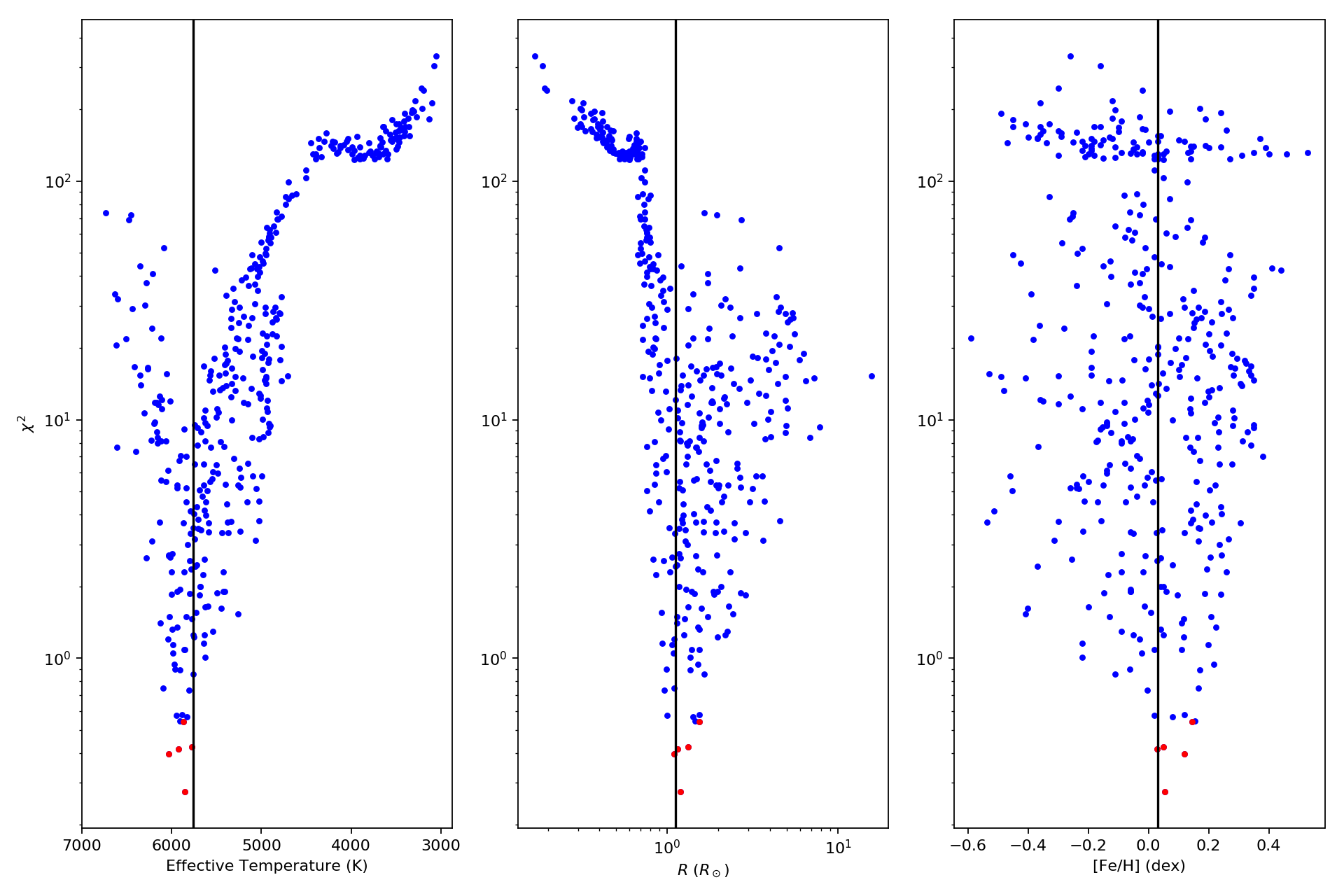
We see that the code does a good job in finding the library stars which are close to parameter space to the target star.
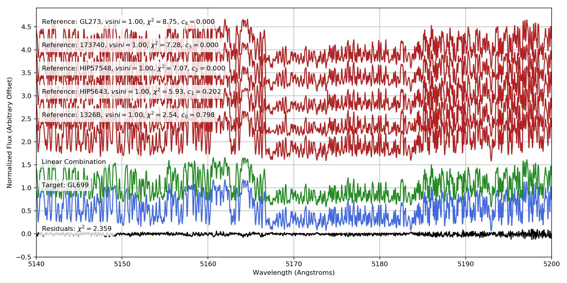
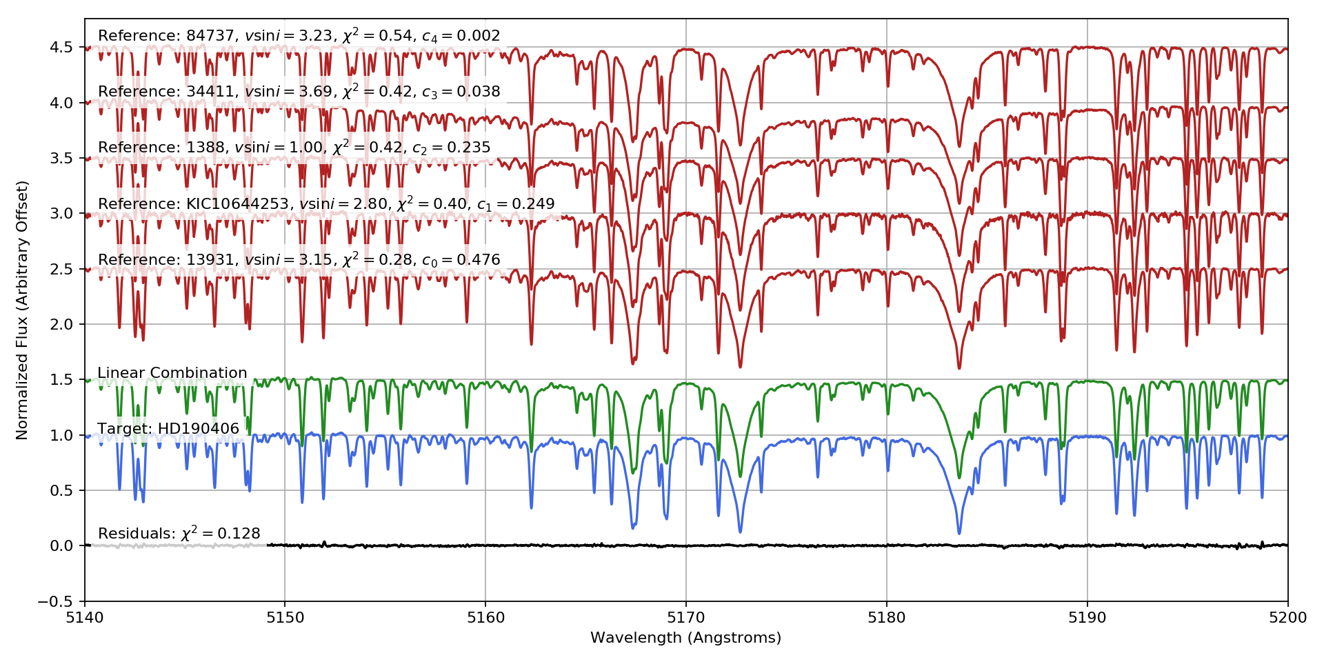
Next, running SpecMatch.lincomb(), the code synthesizes linear
combinations of the best matching spectra to obtain an even better match
to the target.
The respective coefficients will be used to form a weighted average of the library parameters, which are taken to be the derived properties of the target. These are stored in the results attribute.
sm_G.lincomb()

print('Derived Parameters: ')
print('Teff: {0:.0f}, Radius: {1:.2f}, [Fe/H]: {2:.2f}'.format(
    sm_G.results['Teff'], sm_G.results['radius'], sm_G.results['feh']))
print('Library Parameters: ')
print('Teff: {0:.0f}, Radius: {1:.2f}, [Fe/H]: {2:.2f}'.format(
    G_star[0]['Teff'], G_star[0]['radius'], G_star[0]['feh']))
Derived Parameters:
Teff: 5911, Radius: 1.17, [Fe/H]: 0.08
Library Parameters:
Teff: 5763, Radius: 1.11, [Fe/H]: 0.03
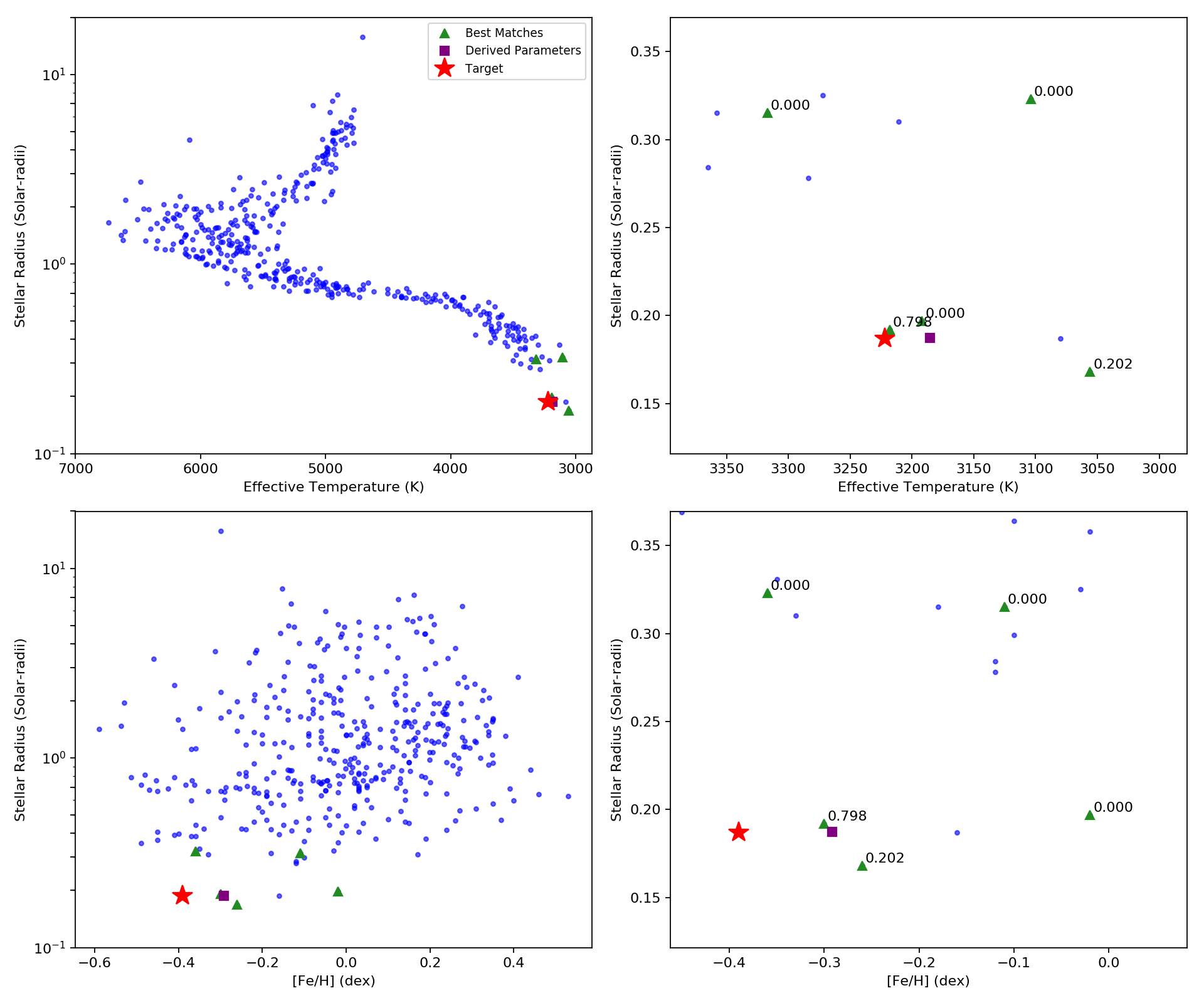
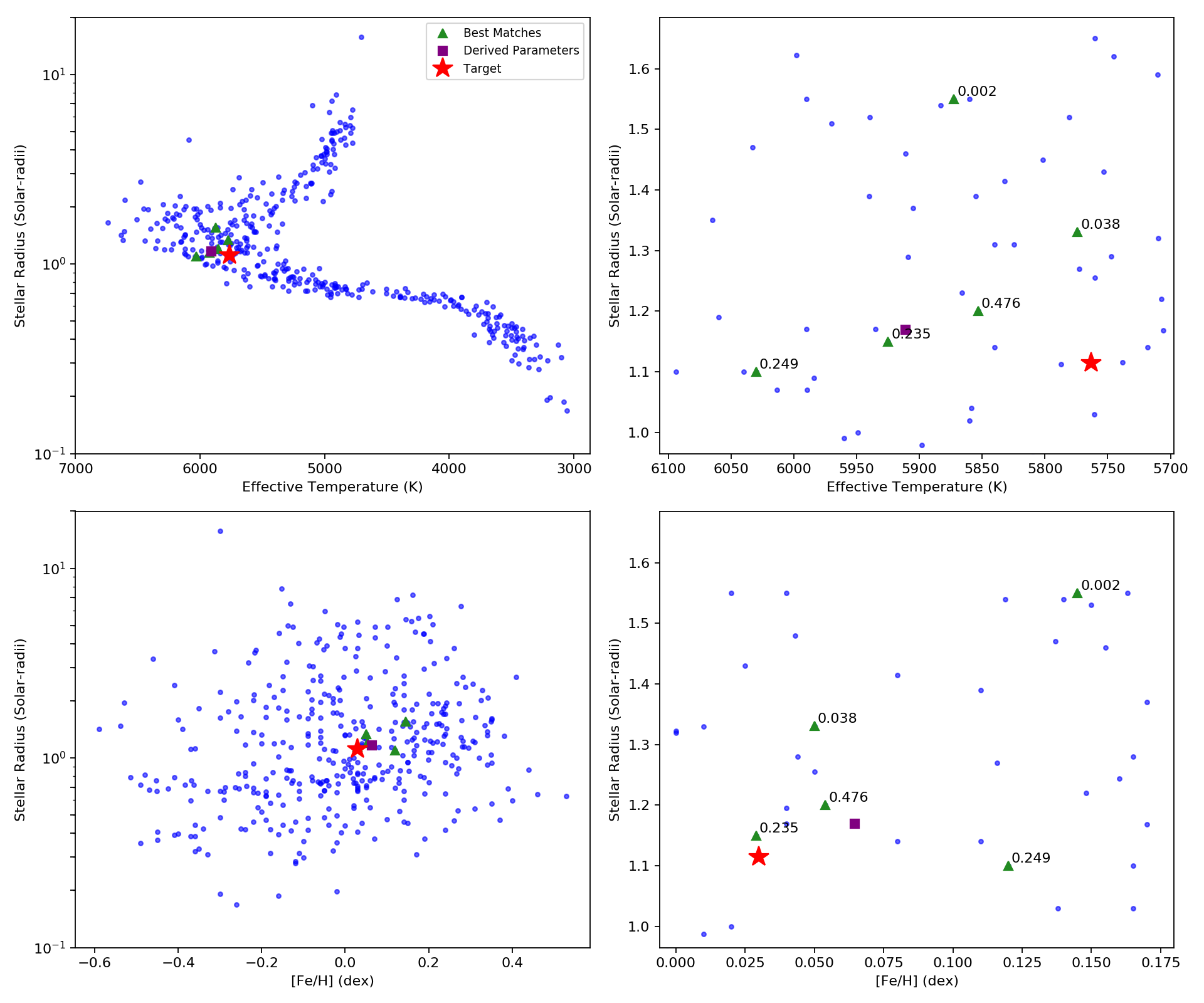
We can take a closer look at the workings of this process by plotting the positions of the best matching library stars in a HR diagram, as well as their spectra.
# Plot HR diagram
fig1 = figure(figsize=(12, 10))
sm_G.plot_references(verbose=True)
# plot target onto HR diagram
axes = fig1.axes
axes[0].plot(G_star[0]['Teff'], G_star[0]['radius'], '*', ms=15, color='red', label='Target')
axes[1].plot(G_star[0]['Teff'], G_star[0]['radius'], '*', ms=15, color='red')
axes[2].plot(G_star[0]['feh'], G_star[0]['radius'], '*', ms=15, color='red')
axes[3].plot(G_star[0]['feh'], G_star[0]['radius'], '*', ms=15, color='red')
axes[0].legend(numpoints=1, fontsize='small', loc='best')


# Plot reference spectra and linear combinations
fig2 = plt.figure(figsize=(12,6))
sm_G.plot_lincomb()
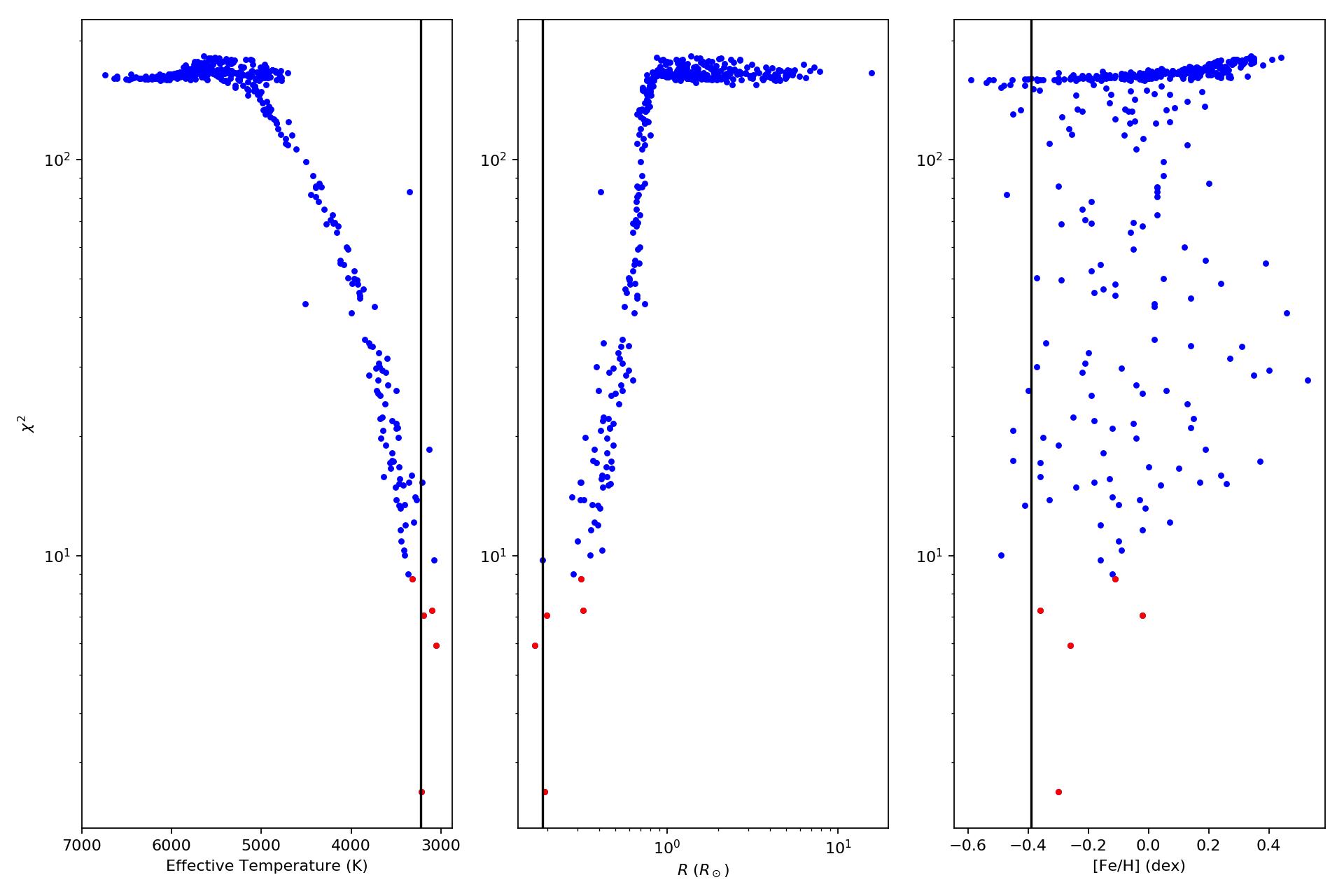
Finally, we can repeat the whole process with Barnard’s star.
# Perform match
sm_M.match(wavlim=(5140,5200))

# Plot chi-squared surfaces
fig1 = figure(figsize=(12,8))
sm_M.plot_chi_squared_surface()
# Indicate library parameters for target star.
axes = fig1.axes
axes[0].axvline(M_star[0]['Teff'], color='k')
axes[1].axvline(M_star[0]['radius'], color='k')
axes[2].axvline(M_star[0]['feh'], color='k')

# Perform lincomb
sm_M.lincomb()

print('Derived Parameters: ')
print('Teff: {0:.0f}, Radius: {1:.2f}, [Fe/H]: {2:.2f}'.format(
    sm_M.results['Teff'], sm_M.results['radius'], sm_M.results['feh']))
print('Library Parameters: ')
print('Teff: {0:.0f}, Radius: {1:.2f}, [Fe/H]: {2:.2f}'.format(
    M_star[0]['Teff'], M_star[0]['radius'], M_star[0]['feh']))

# Plot HR diagram
fig2 = figure(figsize=(12,10))
sm_M.plot_references(verbose=True)
# plot target onto HR diagram
axes = fig2.axes
axes[0].plot(M_star[0]['Teff'], M_star[0]['radius'], '*', ms=15, color='red', label='Target')
axes[1].plot(M_star[0]['Teff'], M_star[0]['radius'], '*', ms=15, color='red')
axes[2].plot(M_star[0]['feh'], M_star[0]['radius'], '*', ms=15, color='red')
axes[3].plot(M_star[0]['feh'], M_star[0]['radius'], '*', ms=15, color='red')
axes[0].legend(numpoints=1, fontsize='small', loc='best')

# Plot reference spectra and linear combinations
fig3 = plt.figure(figsize=(12,6))
sm_M.plot_lincomb()
Derived Parameters:
Teff: 3185, Radius: 0.19, [Fe/H]: -0.39
Library Parameters:
Teff: 3222, Radius: 0.19, [Fe/H]: -0.39